Do females live longer than males?

It is well known that females live longer than males, but does that statement hold statistically? Matthew Martinez and I set out to find out.

Population and the hypothesis

Our population of concern is citizens of the United States. We found a dataset on WorldLifeExpectancy listing by county the average life expectancy for both males and females. With this we form our null and alternative hypothesis

H0: The average life expectancy for both males and females are the same in the United States

HA: The average female life expectancy is higher than the average male life expectancy in the United States

Data preparation

Since the website gives us an overlook at all of the counties in the United States we want to take a small sample of that so we can perform statistics. Using the entire dataset will result in looking at population parameters which doesn’t leave room for inference.

A random number was chosen to pick the state and then the county. This was done a total of 101 times. The CSV file is located here for convenience.

R Programming

For the rest of this article, we will use R for analysis. This article will focus more on the analysis, however, than the R code.

Read the CSV file into R

rm(list=ls())
# Read in file
LifeExpectancy = read.csv("~/LifeExpectancy.csv")
maleExpectancy = LifeExpectancy$Life.Expectancy.Male
femaleExpectancy = LifeExpectancy$Life.Expectancy.Female

Summary Statistics

Before we begin our inferential statistics, it is a good idea to look at what we have in our sample. It will give us a good feeling for what we’re working with and help us answer some questions involving the assumptions in parametric tests.

We’re interested in the minimum, mean, maximum, and interquartile range of the data

# Summary statistics
male_row = c(min(maleExpectancy), mean(maleExpectancy), max(maleExpectancy), IQR(maleExpectancy))
female_row = c(min(femaleExpectancy), mean(femaleExpectancy), max(femaleExpectancy), IQR(femaleExpectancy))
summary = rbind(male_row, female_row)
colnames(summary) = c("Min", "Mean", "Max", "IQR")
rownames(summary) = c("Male", "Female")

Looking at the table below, we can see that the average male lives to be around 69 years old in our sample while the average female lives to be about 71 years old. One interesting thing to note is how small the variation is between all the counties life expectancy that we sampled.

summary
##         Min   Mean  Max   IQR
## Male   69.0 74.952 80.9 2.775
## Female 76.1 80.416 84.1 2.350</code></pre>

Inferential Statistics

From here on out, we will perform a hypothesis test on the two hypothesis stated earlier in the text.

Since our data is quantitative in nature, we will attempt to perform a two sample t-test

Check for Assumptions

Performing a t-test comes with several assumptions we need to check before confidently reporting our results.

Independence Condition: One county’s life span does not affect the lifespan of another.

Independent groups assumption: The lifespan of a male does not directly impact a lifespan of a female.

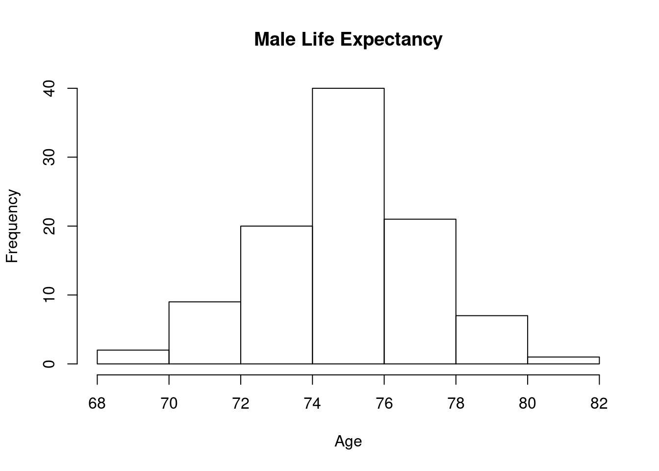
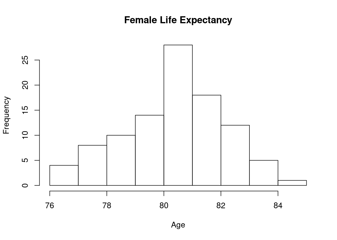
Nearly Normal Condition: We need to check the histograms to see if they’re unimodal and symmetric and check to see if any outliers exist

The male life expectancy distribution appears to be unimodal and symmetric.

# Check for normality
hist(maleExpectancy, main = "Male Life Expectancy", xlab = "Age")

Same with the female life expectancy distribution

hist(femaleExpectancy, main = "Female Life Expectancy", xlab = "Age")

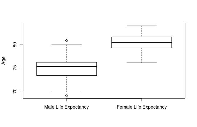
Looking at the boxplot, we can see that the IQR of the female life expectancy is higher than the one of the males. The hypothesis test will show us if this is of significant difference. On the male’s side there are two outliers. This violates the Nearly Normal Condition so we must proceed with caution in our test.

boxplot(maleExpectancy, femaleExpectancy, names = c("Male Life Expectancy", "Female Life Expectancy"), ylab = "Age")

Since the nearly normal condition was not met, we do not meet the assumptions necessary to perform a t-test. However, since the condition was violated by an outlier, let us perform a t-test with the outlier and without the outlier and compare the results.

Calculate the Test Statistic

Let us conduct a two sample t-test with the alternative hypothesis being that the female average life expectancy is greater than that of the males

Running the test below shoes us a p-value of less than 0.001. This tells us that the probability of obtaining a sample as extreme as the one obtained is close to zero. Therefore at a significance level of 5%, we reject the null hypothesis and state that there is strong evidence to suggest that females have a greater life expectancy that that of males.

# Test alternative hypothesis
t.test(femaleExpectancy, maleExpectancy, alternative='g')

##  Welch Two Sample t-test
## 
## data:  femaleExpectancy and maleExpectancy
## t = 18.858, df = 182.48, p-value < 2.2e-16
## alternative hypothesis: true difference in means is greater than 0
## 95 percent confidence interval:
##  4.984992      Inf
## sample estimates:
## mean of x mean of y 
##    80.416    74.952

In fact, we are 95% confident that the difference between the average female life expectancy and the average male life expectancy in the United States is between 5 and 6 years. Females live on average 5-6 years longer than males in the United States.

# Find confidence interval
t.test(femaleExpectancy, maleExpectancy)

##  Welch Two Sample t-test
## 
## data:  femaleExpectancy and maleExpectancy
## t = 18.858, df = 182.48, p-value < 2.2e-16
## alternative hypothesis: true difference in means is not equal to 0
## 95 percent confidence interval:
##  4.892333 6.035667
## sample estimates:
## mean of x mean of y 
##    80.416    74.952

Outlier Analysis

We cannot forget that we had outliers in our dataset. This might affect the results of our test. The point of outlier analysis is to see if such changes are significant.

First let us remove the outliers in R

# Remove outliers
maleExpectancy2 = maleExpectancy[!maleExpectancy %in% boxplot.stats(maleExpectancy)$out]

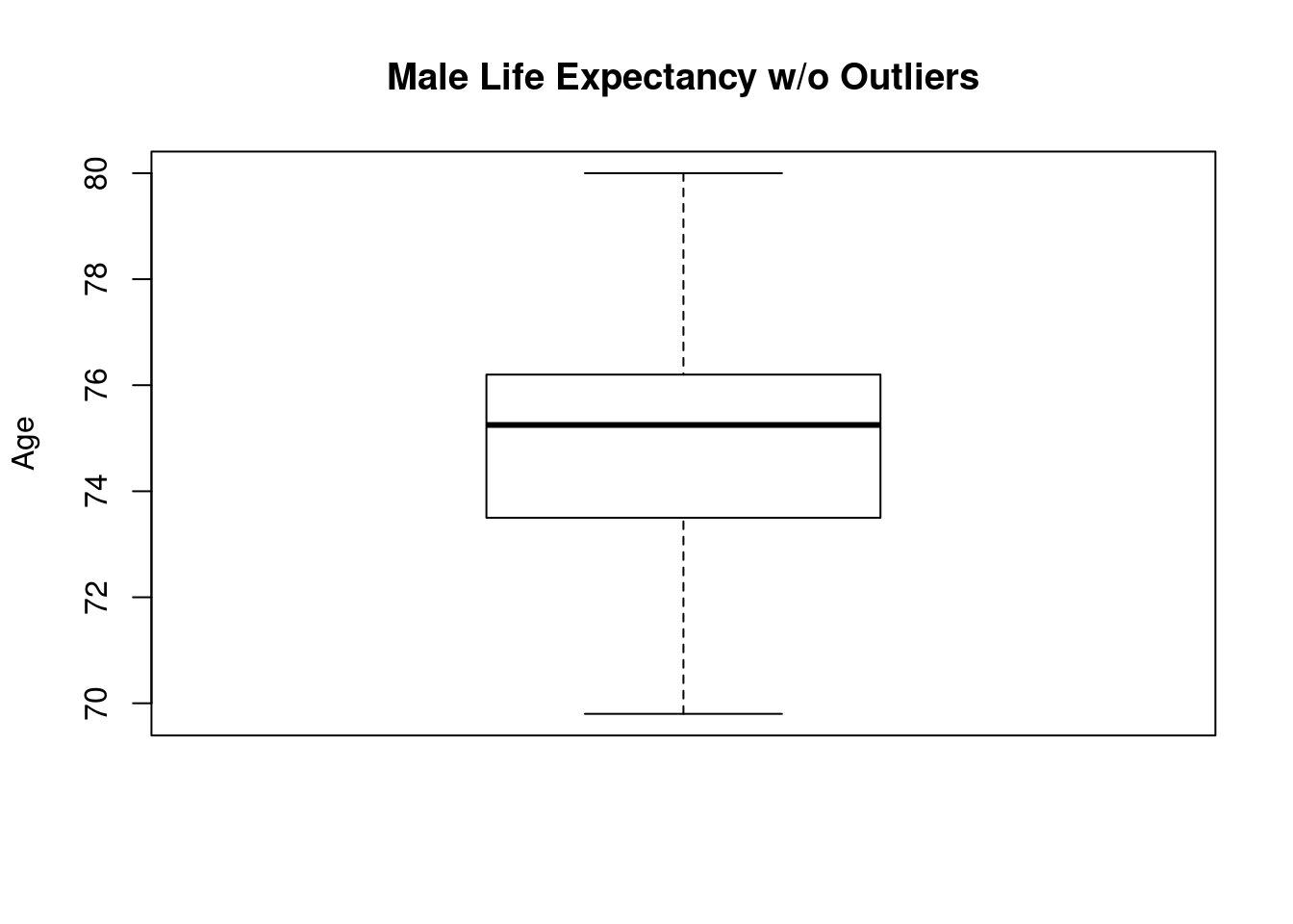
Then let us check the histogram and boxplots to see if the nearly normal condition is now met.

Looking at the boxplot, there are no more outliers present

# Check graphs again
boxplot(maleExpectancy2, ylab = "Age", main = "Male Life Expectancy w/o Outliers")

The histogram still appears to be unimodal and symmetric

hist(maleExpectancy2, xlab = "Age", main = "Male Life Expectancy w/o Outliers")

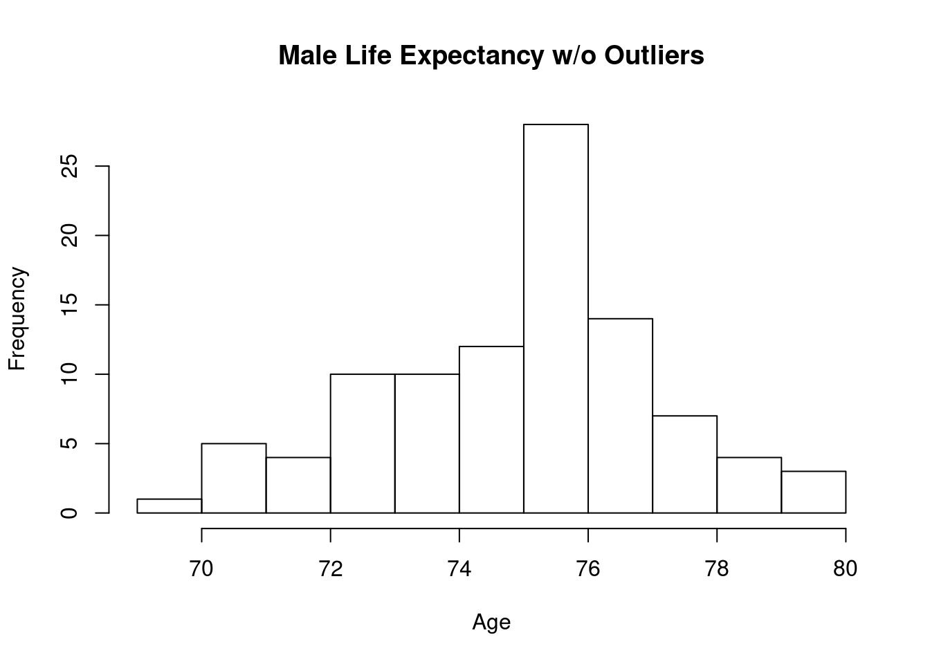
Without the outliers present, the nearly normal condition is now met. We can perform the t-test.

We can see that the hypothesis test returns the same results as before, this tells us that the outliers did not have a significant impact on our test results

# Test new alternative
t.test(femaleExpectancy, maleExpectancy2, alternative='g')

##  Welch Two Sample t-test
## 
## data:  femaleExpectancy and maleExpectancy2
## t = 19.471, df = 184.03, p-value < 2.2e-16
## alternative hypothesis: true difference in means is greater than 0
## 95 percent confidence interval:
##  5.000048      Inf
## sample estimates:
## mean of x mean of y 
##  80.41600  74.95204

Redoing the confidence intervals, we can see that it did not change greatly

# Find new confidence interval
t.test(femaleExpectancy, maleExpectancy2)

##  Welch Two Sample t-test
## 
## data:  femaleExpectancy and maleExpectancy2
## t = 19.471, df = 184.03, p-value < 2.2e-16
## alternative hypothesis: true difference in means is not equal to 0
## 95 percent confidence interval:
##  4.910317 6.017601
## sample estimates:
## mean of x mean of y 
##  80.41600  74.95204

Conclusion

By running the tests and checking the effects of the outliers in the dataset and seeing that the results did not change, we can safely conclude that our interpretations stated before are correct. There is enough evidence to suggest that females in the United States live on average longer than males. We are 95% confident that they live longer than males by 5 to 6 years.