Disc Golf and PyMC3
Published on
Updated on
I’ve been following along with Bayesian Methods for Hackers and I wanted to try using PyMC3 with my own small dataset.
A week ago, a couple friends and I went out and played Disc Golf at a local park. In case you don’t know what Disc Golf is, the goal is for a player to throw a disc at a target with as few throws as possible. Throughout each of the holes, I recorded the number of tosses required until we completed that hole.
| Brandon | Chris | Clare |
|---|---|---|
| 6 | 8 | 10 |
| 7 | 9 | 10 |
| 7 | 8 | 9 |
| 7 | 7 | 8 |
| 5 | 4 | 9 |
| 5 | 5 | 10 |
| 4 | 4 | 7 |
| 5 | 6 | 9 |
| 6 | 5 | 7 |
| 7 | 7 | 8 |
| 5 | 6 | 8 |
| 6 | 5 | 7 |
| 6 | 6 | 8 |
| 5 | 4 | 6 |
You can also download the CSV.
What I want to know is the distribution of the number of tosses for each player.
PyMC3
Let’s try answering this with Bayesian Statistics + PyMC3.
First we’ll need to import the relevant packages
import pandas as pd
import pymc3 as pm
import matplotlib.pyplot as plt
import numpy as np
from scipy.stats import poisson
Load in the data
DISC_DATA = pd.read_csv("data/discgolf03242020.csv")
PEOPLE = ["Brandon", "Chris", "Clare"]
Since the number of tosses are count data, we are going to use the Poisson distribution for the estimation. This means that we are going to characterize each player’s number of tosses with this distribution. The Poisson distribution has a parameter $\lambda$ which also serves as the expected value. The shape of the distribution is dependent on this parameter, so we’ll need to estimate what this parameter is. Since the expected value must be positive, the exponential distribution is a good candidate. $$ toss \sim Poisson(\lambda) \ \lambda \sim Exp(\alpha) $$ The exponential distribution also has a parameter $\alpha$. The expected value of an exponential distribution with respect to $\alpha$ is $\frac{1}{\alpha}$. At this point we can give an estimate of what we believe $\alpha$ could be. Given the relationships with the expected values, the mean score of each of the players is a great choice.
with pm.Model() as model:
    # Random Variables
    ALPHA = [1. / DISC_DATA[person].mean() for person in PEOPLE]
    LAMBDAS = [pm.Exponential("lambda_" + person, alpha) for person, alpha in zip(PEOPLE, ALPHAS)]
Now to show how easy the library is, we will provide the data and run Monte Carlo simulations to see the distribution that the $\lambda$s live in.
with model:
    OBS = [
        pm.Poisson("obs_" + person, lambda_, observed=DISC_DATA[person])
        for person, lambda_ in zip(PEOPLE, LAMBDAS)
    ]
    TRACES = pm.sample(10000, tune=5000)
We can then grab the distribution of $\lambda$s from the trace.
LAMBDA_SAMPLES = [TRACE["lambda_" + person] for person in PEOPLE]
Visualization
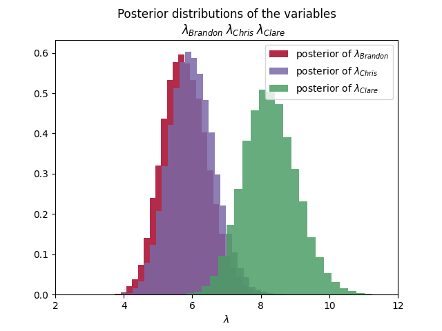
First let’s check out the average disc tosses for each player by looking at how the $\lambda$s are distributed.
plt.figure("Distribution of Average Disc Tosses")
for person, lambda_sample, color in zip(PEOPLE, LAMBDA_SAMPLES, COLORS):
    plt.hist(lambda_sample,
        histtype='stepfilled', bins=30, alpha=0.85,
        label=r"posterior of $\lambda_{" + person + "}$",
        color=color, density=True
    )
PARAMETER_TITLE = r"\;".join(
    [r"\lambda_{" + person + "}" for person in PEOPLE]
)
plt.title(f"""Posterior distributions of the variables
    ${PARAMETER_TITLE}$""")
plt.xlim([
    DISC_DATA[PEOPLE].min().min() - 2,
    DISC_DATA[PEOPLE].max().max() + 2
])
plt.legend()
plt.xlabel(r"$\lambda$")
plt.show()
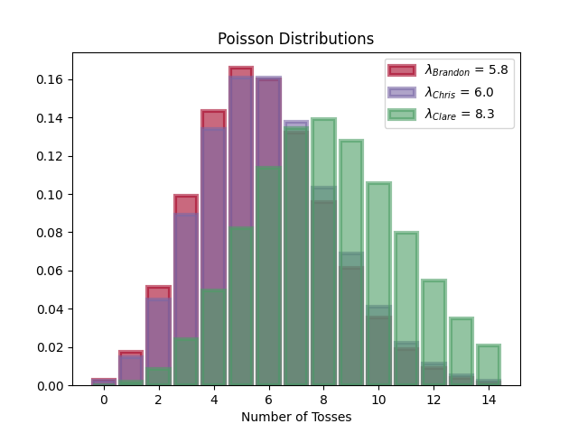
Now let’s look at the distribution of the number of tosses for each player
plt.figure("Distribution of Disc Tosses")
for person, lambda_sample, color in zip(PEOPLE, LAMBDA_SAMPLES, COLORS):
    tosses = np.arange(15)
    lambda_ = lambda_sample.mean()
    plt.bar(tosses, poisson.pmf(tosses, lambda_), color=color,
            label=r"$\lambda_{" + person + "}$ = " + "{:0.1f}".format(lambda_),
            alpha=0.60, edgecolor=color, lw="3"
    )
plt.legend()
plt.xlabel("Number of Tosses")
plt.title("Poisson Distributions")
Conclusion
We can see in the first graphic that the average number of tosses required for Brandon and Chris is about $6$, while for Clare it’s $8$. Looking at the second graphic though, shows us that Clare has a wide range of possible tosses.
With PyMC3, we got to see the larger trends in the data by analyzing distributions that are more likely given the data.
For easy reference, here is the entire script.
import pandas as pd
import pymc3 as pm
import matplotlib.pyplot as plt
import numpy as np
from scipy.stats import poisson

DISC_DATA = pd.read_csv("data/discgolf03242020.csv")
PEOPLE = ["Brandon", "Chris", "Clare"]
COLORS = ["#A60628", "#7A68A6", "#4c9e65"]

assert len(PEOPLE) == len(COLORS)

with pm.Model() as model:
    # Random Variables
    ALPHAS = [1. / DISC_DATA[person].mean() for person in PEOPLE]
    LAMBDAS = [pm.Exponential("lambda_" + person, alpha) for person, alpha in zip(PEOPLE, ALPHAS)]

    # Observations
    OBS = [
        pm.Poisson("obs_" + person, lambda_, observed=DISC_DATA[person])
        for person, lambda_ in zip(PEOPLE, LAMBDAS)
    ]

    # Monte-Carlo
    TRACE = pm.sample(10000, tune=5000)

LAMBDA_SAMPLES = [TRACE["lambda_" + person] for person in PEOPLE]

# Graph histogram of samples
plt.figure("Distribution of Average Disc Tosses")
for person, lambda_sample, color in zip(PEOPLE, LAMBDA_SAMPLES, COLORS):
    plt.hist(lambda_sample,
        histtype='stepfilled', bins=30, alpha=0.85,
        label=r"posterior of $\lambda_{" + person + "}$",
        color=color, density=True
    )
PARAMETER_TITLE = r"\;".join(
    [r"\lambda_{" + person + "}" for person in PEOPLE]
)
plt.title(f"""Posterior distributions of the variables
    ${PARAMETER_TITLE}$""")
plt.xlim([
    DISC_DATA[PEOPLE].min().min() - 2,
    DISC_DATA[PEOPLE].max().max() + 2
])
plt.legend()
plt.xlabel(r"$\lambda$")

# Graph Poisson Distributions
plt.figure("Distribution of Disc Tosses")
for person, lambda_sample, color in zip(PEOPLE, LAMBDA_SAMPLES, COLORS):
    tosses = np.arange(15)
    lambda_ = lambda_sample.mean()
    plt.bar(tosses, poisson.pmf(tosses, lambda_), color=color,
            label=r"$\lambda_{" + person + "}$ = " + "{:0.1f}".format(lambda_),
            alpha=0.60, edgecolor=color, lw="3"
    )
plt.legend()
plt.xlabel("Number of Tosses")
plt.title("Poisson Distributions")

plt.show()